Pose Sketching for the Control of a Humanoid Robot - Part 2

Introduction

In this series of posts, I will be writing up about some work done in the context of a semester project counting for my degree from EPFL. This is meant more as a record than an in-depth tutorial, but don’t hesitate to drop me a line if you would like to see more details. This work was done under supervision by Sylvain Calinon, senior researcher in the Robot Learning & Interaction Group at Idiap Research Institute in Martigny, Switzerland.

The main focus of the project was to investigate new ways of controlling high degree of freedom robots, with an application to the Humanoid robot Baxter.

Visual servoing

Visual servoing, or vision-based control, uses visual feedback to control a robot. In particular, eye-in-hand, or end-point open-loop control is a setting where the camera is free and tracks the relative position of the arm with respect to the points in the world coordinates.

We intend to apply here a version of visual servoing in which the control law is based on minimising the error between the observed pose and the desired pose by minimising the error in the image (i.e. working in the pixel space directly). This is called Image-Based Visual Servoing (IBVS) proposed by Weiss et al. ¹.

Mapping the task space to the pixel space

As is often the case in control settings, we need to find a mapping between different coordinate spaces since the commands to the robot are given in its own local referential (the joint angles) but the effects of these commands (e.g. moving the arm) are to be measured in the global referential (for example xyz coordinates of the robot’s end-effector) if they are to have any relevance to the task at hand.

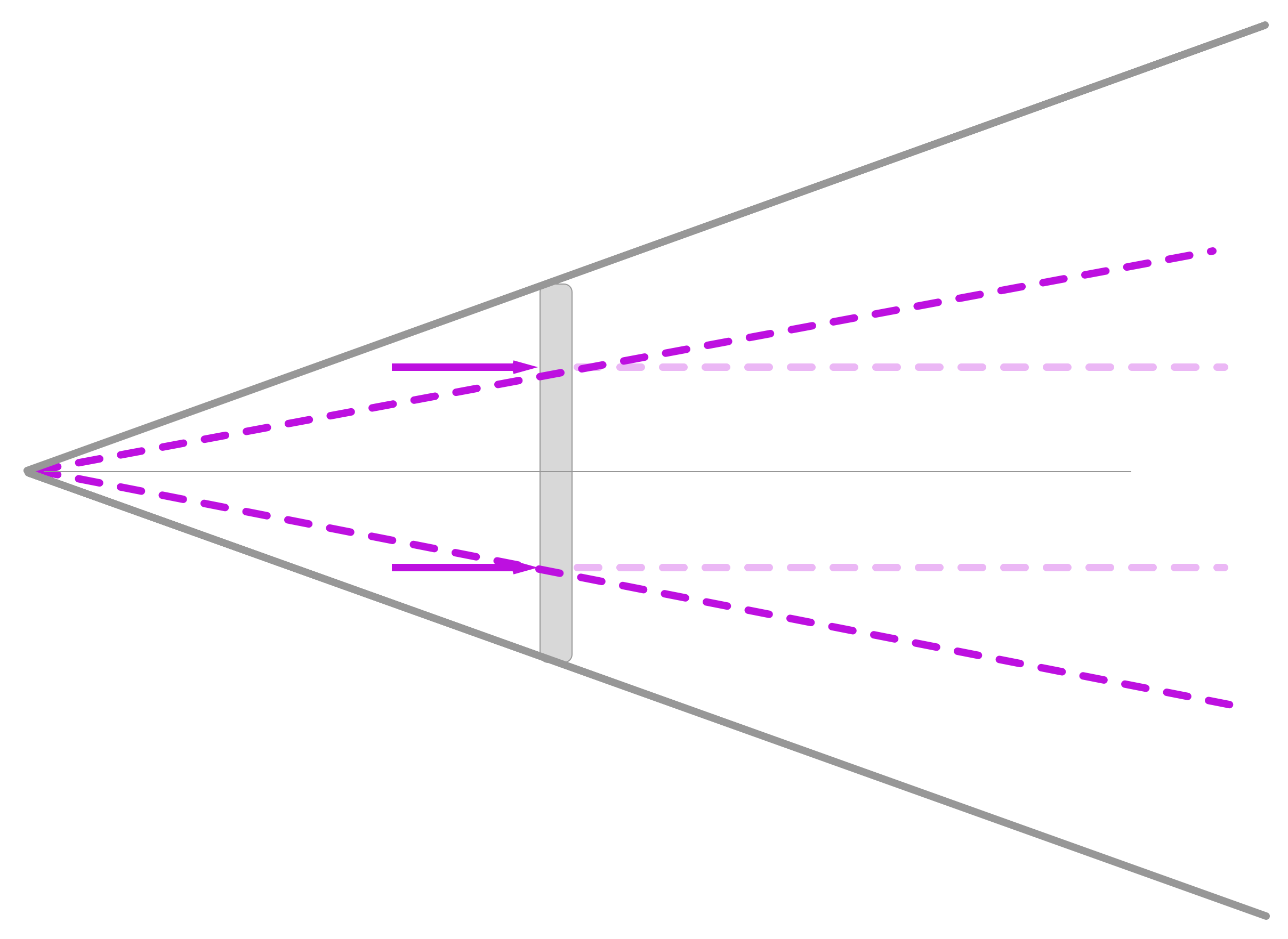
Figure 1: Linearised optical model

Since our objective is to have a map between any pixel on our interface and points in the real world (what point in the real world is this pixel showing me, hence if I click on this pixel, what point in the real world am I interacting with ?). Obviously the difficulty resides in the fact that there is not a unique solution in the real world for each pixel on the interface. This is already obvious with a simple ray-tracing model. Take a pixel on the screen and trace a straight line forward from the interface. Every single point on this line is mapped to the same pixel on the screen so there is no way (for now) to know which of these points we were aiming for when clicking on this pixel. One way to get around this problem is to trace not one but two lines, coming from the interface at different positions but from the same point on the interface. The intersection of these two lines defines a unique point in space for this pixel.

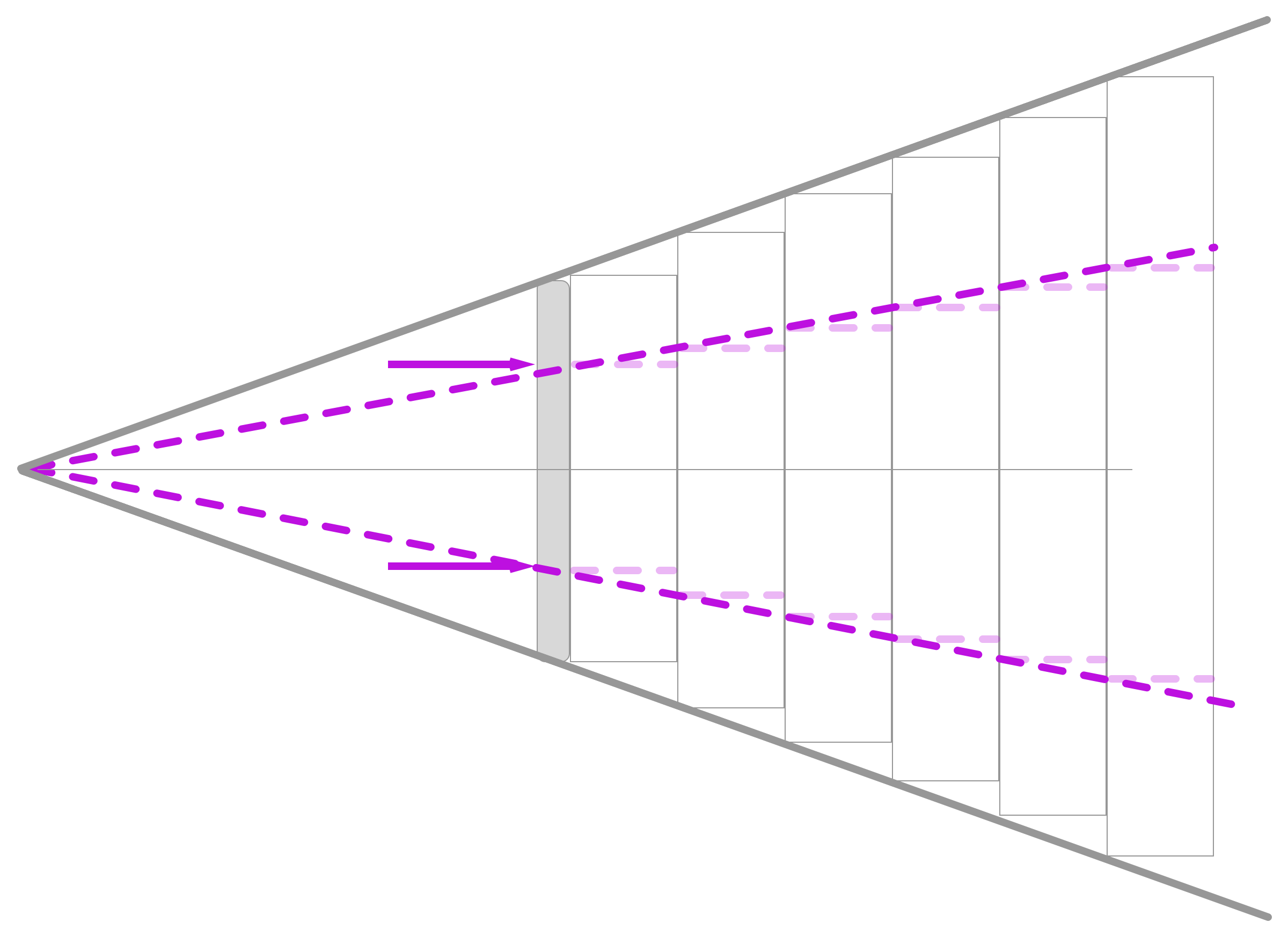
Figure 2: Piece-wise linearised optical model

This ray-tracing method is the simplest way to get a mapping from point to pixel and is quite useful for experimentation in a simple setting. Unfortunately it is unusable in a real setting, simply because this is not at all how lenses work, with the error of this model growing quadratically with the distance to the interface. It assumes there is a 1-1 mapping in scale between the screen and the objects (no distortion, no magnification), where using a lens allows us to view large scenes on a small screen. To circumvent this we can use a pinhole camera model that projects straight lines from a focal point behind the interface, but this also assumes the absence of distortion. We could also apply some form of linearisation which approximates this simple camera model but provides an easer geometrical framework (piece-wise linear) by stacking arbitrarily thin chunks of rays.

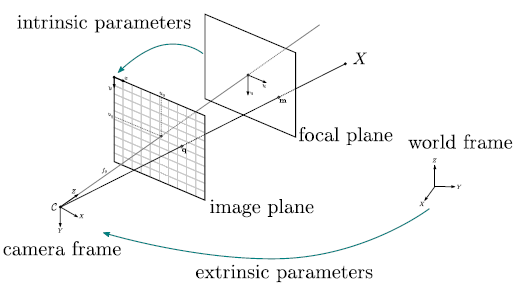
Figure 3: Pinhole camera model

Thankfully, optics provides us with a simple way to get over these issues by defining a projective matrix for the optical system of the camera. All we need to know are some basic lens characteristics: $f_x$ and $f_y$ are the respective focal lengths on axis x and y of the lens, $s$ is the axis skew (which causes distortion in the image), $x_0$ and $y_0$ are the displacements of the studied point (in our case, where the user clicked on the screen). Note that these parameters are expressed in pixel units, meaning the distances are not taken into account. To model this dependency we can use a scaled version, dividing the values by the factor of the sensor sizes in pixels and mm.

$$\mathbf{K} = \begin{bmatrix} f_x & s & x_0 \\ 0 & f_y & y_0 \\ 0 & 0 & 1 \end{bmatrix}$$

However, this method is incomplete. We only get the matrix $K$ which models the lens, and not the camera. For this we simply incorporate an extrinsic matrix (as opposed to the intrinsic matrix $\mathbf{K}$), modelling the pose of the camera in the world space, in generalised coordinates, comprised of a rotation $\mathbf{R}$ and a translation $t$.

$$\mathbf{P} = \mathbf{K} \cdot \begin{bmatrix} \mathbf{R} | t \end{bmatrix} \,\,\,\,,$$

Some methods have been proposed to learn such a mapping, such as deriving it online as in ², or by calibrating the system with a point known by both the robot and the camera (getting an intermediate referential). In practice, this is the simplest way to find it. In our experiments we calibrated with the robot’s end effector as a known position, but previous attempts have defined arbitrary intermediate referentials for calibration.

Controlling the robot from the pixel space

So once we have learnt these maps, we can finally use them to do something useful (well, at least fun): moving robots around ! Let’s define a simple robot as in Fig. 4. The arm of the robot is defined by two joint angles ($\mathbf{q} = [q_1\, \,q_2]^T$), and the end-effector’s position in the robot space is denoted $\mathbf{x_R}$.

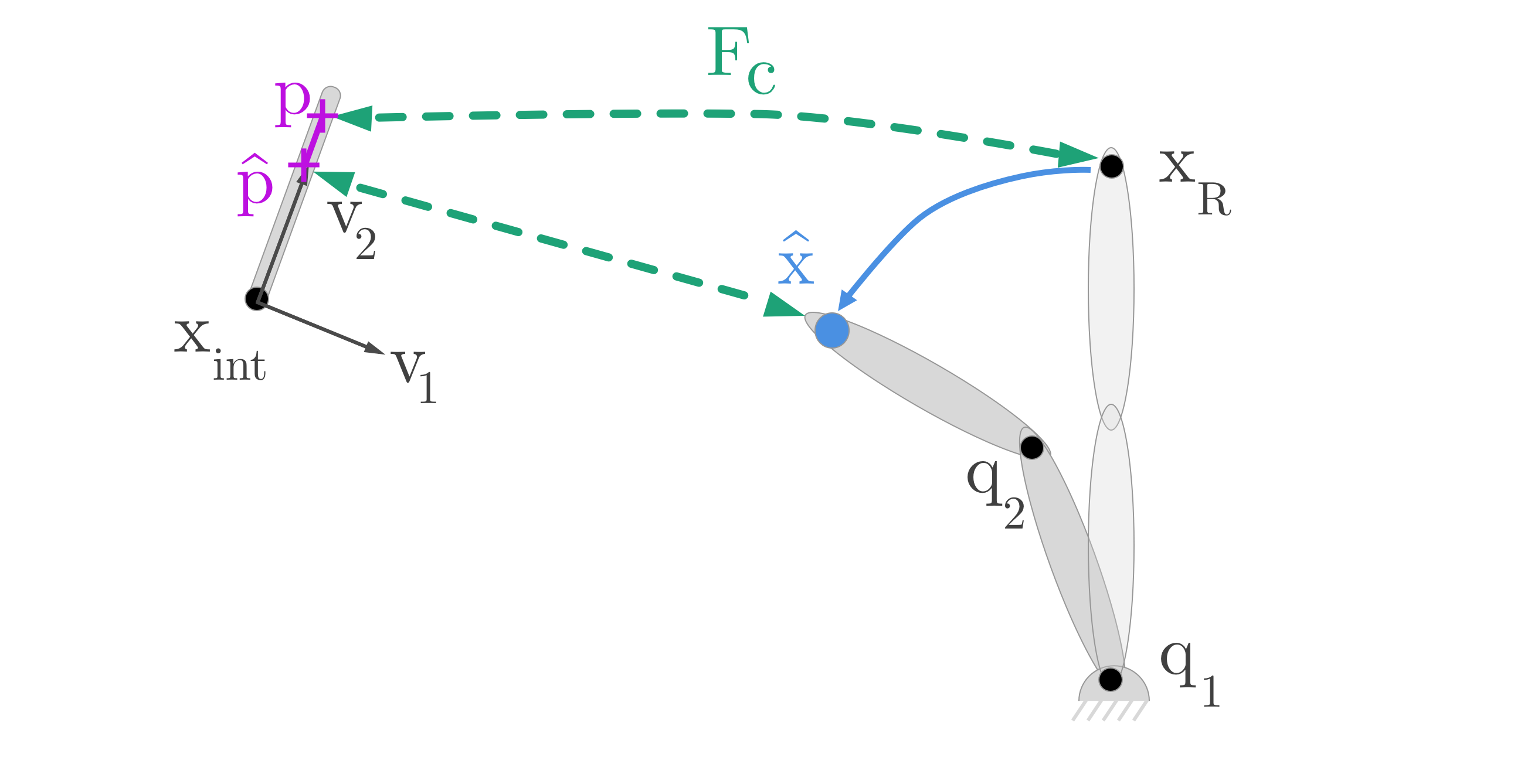
Figure 4: Controlling in the pixel space

Following our previous argument, we learn a mapping $F_c$ which brings a point $\mathbf{x}$ in world space to a point $\mathbf{p}$ in the pixel space (on the screen). We could use the simple method of ray-tracing but as detailed earlier this method has severe shortcomings.

$$F_c(\mathbf{x_R}) = \mathbf{p}$$

We also need to know how the end-effector get its position based on the joint angles of the robot. This is the kinematic model of the robot, and can be formalized as:

$$F(\mathbf{q}) = \mathbf{x_R}$$

Well the rest is now straighforward: we have two mappings: one to go from the joint angles (what we want to control) to the end-effector’s position in space, and another from the end-effector onto the screen. We can compose the two to get a direct relationship between a position on the screen and a joint angle !

$$\mathbf{p} = F_c(F(\mathbf{q}))$$

We can now define a control law that will minimise the error in the pixel space between the desired position $\hat{\mathbf{p}}$ and the current position $\mathbf{p}$ by controlling the joint angles $\mathbf{q}$. This can be obtained by applying the chain rule to the previous mapping, to obtain:

$$\begin{align} \frac{\partial{\mathbf{p}}}{\partial{\mathbf{q}}} &= \frac{\partial ({F_c \circ F}) }{\partial{\mathbf{q}}} \\ & = \frac{\partial F}{\partial \mathbf{q}} \cdot \frac{\partial F_c}{\partial \mathbf{q}} \Bigg\rvert_{F(\mathbf{q})} \\ & = \mathbf{J} \cdot \mathbf{J}_c \big\rvert_{F(\mathbf{q})} \end{align}$$

where $\mathbf{J}$ is the Jacobian of $F$, mapping velocities from the joint-angles to the end-effector, and $\mathbf{J_c}$ is the Jacobian of $F_c$, mapping velocities from the end-effector to the pixel space. The final control law is obtained by computing the pseudo-inverse ($^+$) of this relation to finally get, for a simple PD controller (the gain $k_p$ controls how aggressively we want to reach the solution):

$$\dot{\mathbf{q}} = (\mathbf{J} \cdot \mathbf{J}_c \big\rvert_{F(\mathbf{q})} )^{+} \cdot k_p (\mathbf{p} - \hat{\mathbf{p}})$$

Visual servoing with Baxter

We now have everything at our disposal to use this in the real world. We implemented the ideas developed earlier in the context of an Android app, running Tango (RIP) for the visual part, and ROS to communicate with the Baxter robot. After many hurdles, there is finally a cool video to show.

Intrinsic matrix and Camera parameters

As we have seen the intrinsic matrix is entirely defined by camera parameters. In our case we were able to retrieve them from Tango, letting us plugin the desired values to the matrix $\mathbf{K}$.

Extrinsic matrix and Calibration

We also have to learn the extrinsic matrix so we can figure out where the camera and robot are relative to each other. For this we used the simplest method available: since the phone’s pose as given by Tango was relative to the start-up position, we simply start-up the app at a position that is known from the robot, such as its end-effector. We can see this step in Fig. 5.

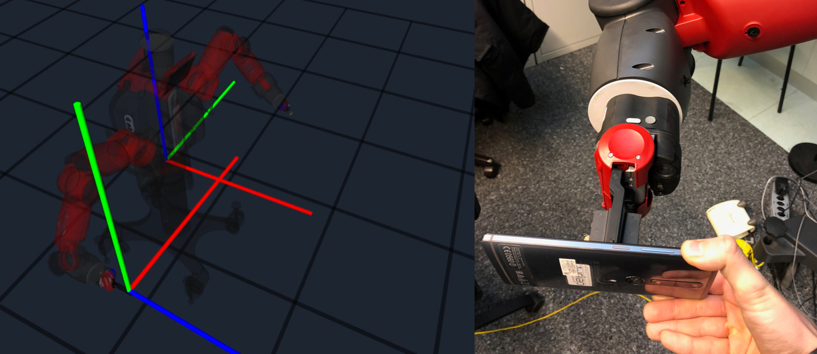
Figure 5: Calibration step

Visual interaction

We can now click on the interface to give the robot commands. The pipeline we described computes a direct mapping from the clicked position to joint angles. As mentioned there can be several solutions to the inverse map, so it is sometimes necessary to define several points, with there solutions being averaged out to give the final command for the end-effector.

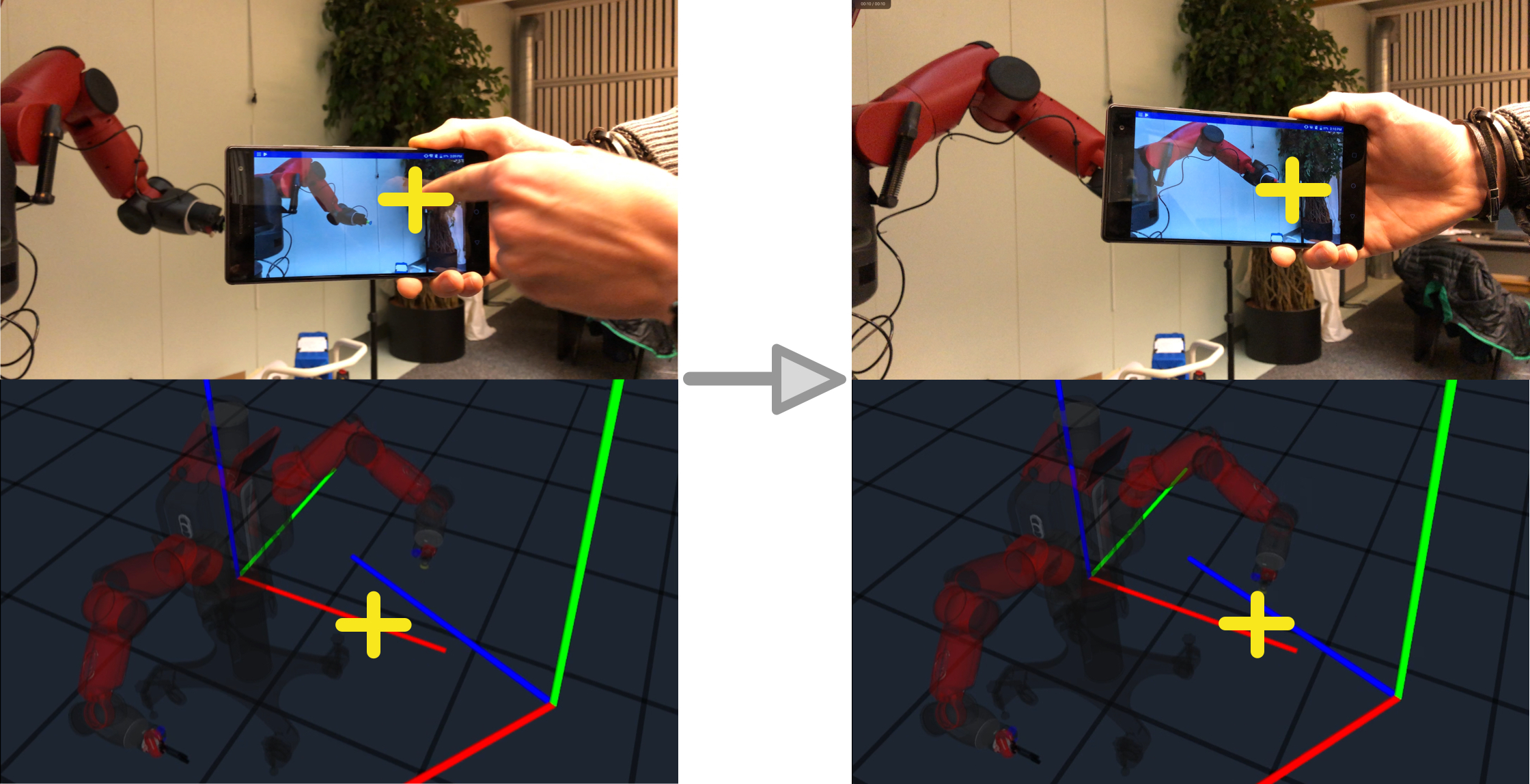
Figure 6: Controlling in the pixel space

Final thoughts

We present here a way of controlling the robot using information directly on the device (controlling in the pixel space), which opens a new set of intersecting control methods but also providing feedback in the same space as the interaction. This write-up is far from extensive and needs quite a bit of refining, but I hope you found it fun to follow along.

If you find mistakes, have comments or concerns, don’t hesitate to ping me !

I’d really like to thank Sylvain Calinon for supervising me during this project, as well as Emmanuel Pignat who really helped salvage the results.

Resources

The code for the Android application is available on Gitlab. The presentation of this work can be found on Youtube, where I describe in a bit more detail the work that was done at IDIAP. If you are very interested, the final report for this project is also available. All of this surely needs a lot of improvements, but that’s what we’re all here for aren’t we ? :)

---